How to Calibrate a Magnetometer?
Magnetometers are used to measure the strength of a magnetic field. They can also be used to determine orientation and to compensate gyro drift. Magnetometer provides the last three degrees of freedom in 9DOF sensors.
There is one problem though, magnetometers are prone to distortion.
Hard iron distortion
The magnetic field used for determining the heading is the earth’s magnetic field. In addition to earth’s, there are additional magnetic fields which cause interference. Interference can be caused by ferromagnetic material or equipment in the magnetometers vicinity. If the magnetic field is permanent it is called “hard iron”.
For example a mobile phone has a speaker. The speaker is permanently attached to the phone. Because of this the location and the orientation of the speakers magnetic field does not change over time. For the magnetometer inside the phone the speaker is considered hard iron.
Good thing about hard iron bias is that it can be easily corrected. Hard iron distortion is always additive to the to the earth’s magnetic field. In other words sensor reading can be corrected ie. unbiased by simply removing the offset. Pseudocode for removing the offset would be something like the following.
offset_x = (max(x) + min(x)) / 2
offset_y = (max(y) + min(y)) / 2
offset_z = (max(z) + min(z)) / 2

corrected_x = sensor_x - offset_x
corrected_y = sensor_y - offset_y
corrected_z = sensor_z - offset_z
Soft iron distortion
Soft iron distortion is the result of material that distorts a magnetic field but does not necessarily generate a magnetic field itself. For example iron (the metal) will generate a distortion but this distorion is dependent upon the orientation of the material relative to the magnetometer.
Unlike hard iron distortion, soft iron distortion cannot be removed by simply removing the constant offset. Correcting soft iron distortion is usually more computation expensive and involves 3x3 transformation matrix.
There is also a computatively cheaper way by using scale biases as explained by Kris Winer. This method should also give reasonably good results. Example pseudocode below includes also the hard iron offset from the previous step.
avg_delta_x = (max(x) - min(x)) / 2
avg_delta_y = (max(y) - min(y)) / 2
avg_delta_z = (max(z) - min(z)) / 2

avg_delta = (avg_delta_x + avg_delta_y + avg_delta_z) / 3

scale_x = avg_delta / avg_delta_x
scale_y = avg_delta / avg_delta_y
scale_z = avg_delta / avg_delta_z

corrected_x = (sensor_x - offset_x) * scale_x
corrected_y = (sensor_y - offset_y) * scale_y
corrected_z = (sensor_z - offset_z) * scale_z
Capture some sensor data
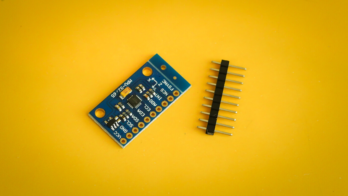
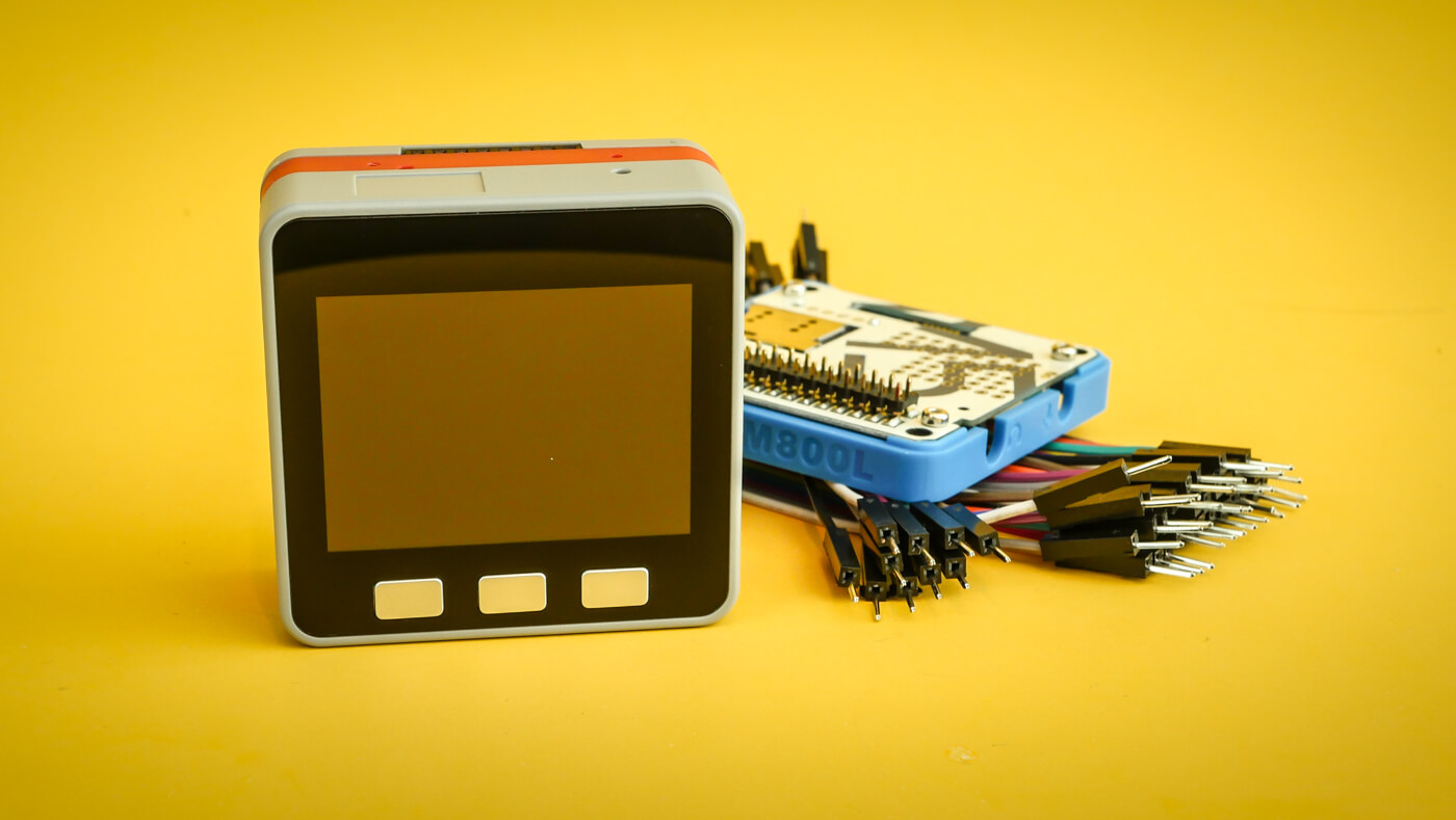
Visualizing the data helps to understand it. It also helps to see the differences after calibrating. For capturing I used the [M5Stack MPU9250 4MB][3] which as the name suggest has a MPU-9250 9DOF sensor inside.
MPU-9250 is a System in Package (SiP) which combines two chips: MPU-6500 which contains 3-axis gyroscope and 3-axis accelerometer and an AK8963 which is a 3-axis digital compass.
Sensor readings are outputted using a MicroPython script to the serial console. Script uses an I2C MPU-9250 driver. After starting the script move the sensor in a big figure eight. Basically the same what you did as a child when playing with toy aeroplane. The sensor should rotate multiple times around the X, Y and Z axles.
import micropython
import utime
from machine import I2C, Pin, Timer
from mpu9250 import MPU9250

micropython.alloc_emergency_exception_buf(100)

i2c = I2C(scl=Pin(22), sda=Pin(21))
sensor = MPU9250(i2c)

def read_sensor(timer):
    value = sensor.magnetic
    print(",".join(map(str, value)))

timer_0 = Timer(0)
timer_0.init(period=500, mode=Timer.PERIODIC, callback=read_sensor)
After approximately 1-2 minutes of waving, copy paste the sensor readings from the console to a csv file. Let’s call it magnetometer.csv. The more data you capture the better.
Seeing is believing
Gnuplot is an excellent cross plaform command line graphing utility. It probably does not appeal to hipster types. There is no unicorn emojis and stuff. It gets the work done though.
If you are on macOS install Gnuplot with Homebrew.
$ brew install gnuplot --with-qt
$ gnuplot
First tell gnuplot input file will be a CSV file.
gnuplot> set datafile separator ","
Scattergraph is good for visualizing magnetometer readings. For three axes we need three separate graphs.
In the plot command using 1:2 states that the values for XY graph are taken from the first and second column. XZ uses data from first and third column, thus using 1:3. YZ is plotted with using 2:3 which are the second and third columns.
gnuplot> plot "magnetometer.csv" using 1:2 title "XY" pointsize 2 pointtype 7, \
              "magnetometer.csv" using 1:3 title "XZ" pointsize 2 pointtype 7, \
              "magnetometer.csv" using 2:3 title "YZ" pointsize 2 pointtype 7
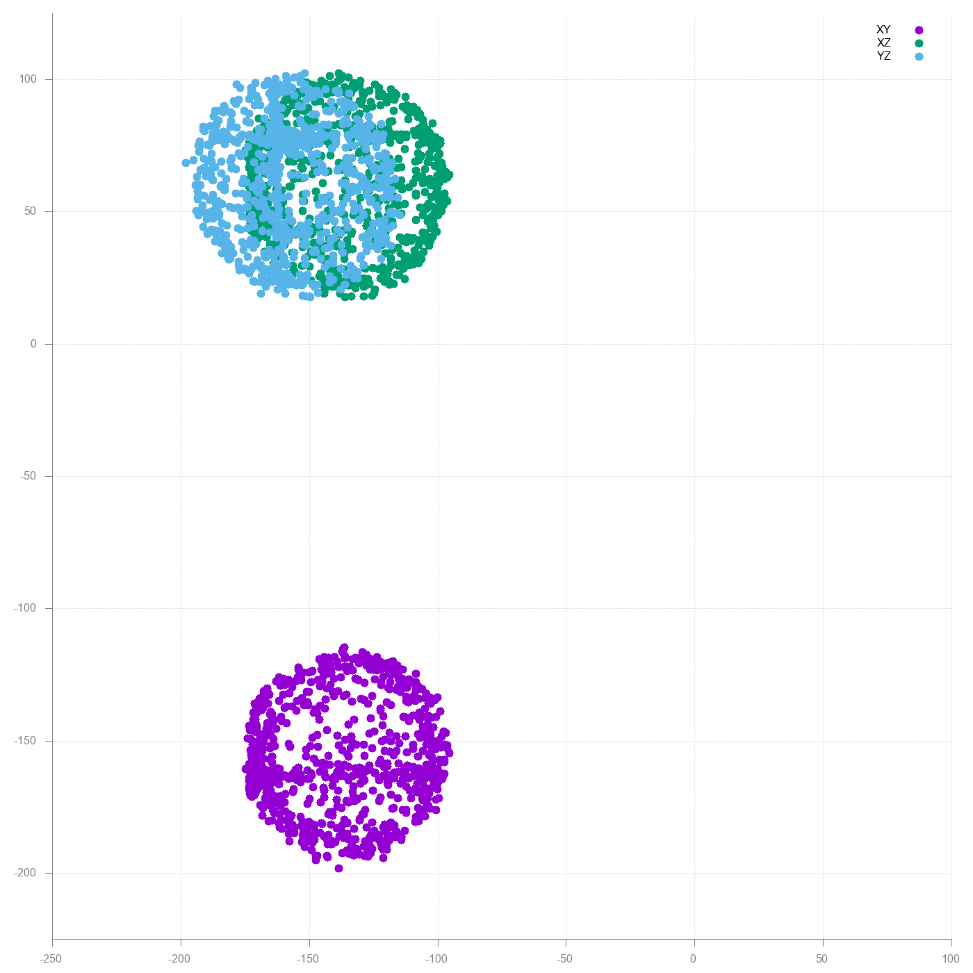
The result should be three similar sized spheres centered around 0,0 coordinates. Here is what I got.
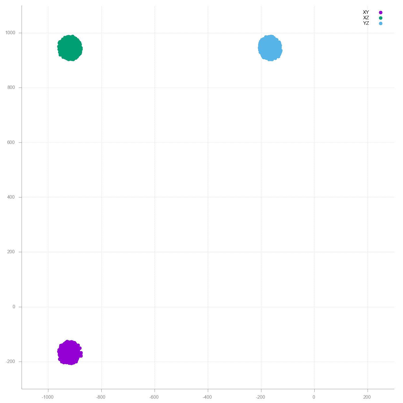
First WTF moment. The graphs do not make any sense. Then I realized M5Stack bottomplate has a magnet which is a schoolbook example of hard iron interference.
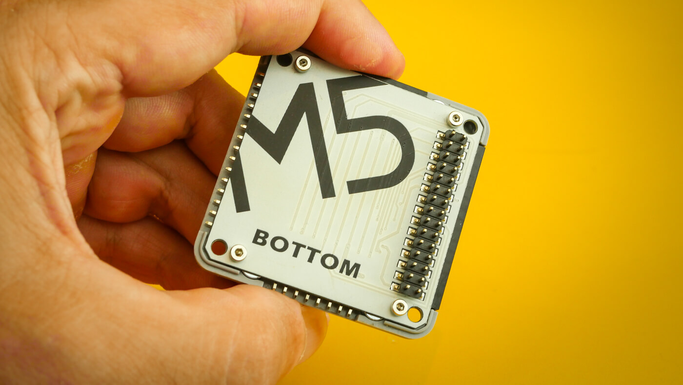
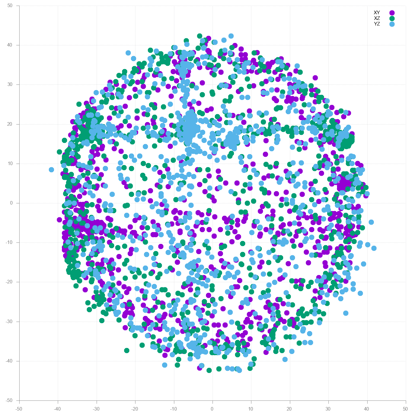
New try with the backplate removed.
Much better, but still a lot of distortion. The big offset is still hard iron distortion. Most likely caused by the loudspeaker inside M5Stack. Below is an implementation hard iron offset removal in Python.
#!/usr/local/bin/python3

import csv
import sys

reader = csv.reader(iter(sys.stdin.readline, ""), delimiter=",")
data = list(reader)

x = [float(row[0]) for row in data]
y = [float(row[1]) for row in data]
z = [float(row[2]) for row in data]

offset_x = (max(x) + min(x)) / 2
offset_y = (max(y) + min(y)) / 2
offset_z = (max(z) + min(z)) / 2

for row in data:
    corrected_x = float(row[0]) - offset_x
    corrected_y = float(row[1]) - offset_y
    corrected_z = float(row[2]) - offset_z

    print(",".join(format(value, ".15f") for value in [corrected_x, corrected_y, corrected_z]))
Run the script to generate new csv file with hard iron distortion corrected.
$ ./hardiron.py < magnetometer.csv > hardiron.csv
Plot new graph using the corrected values.
gnuplot> plot "hardiron.csv" using 1:2 title "XY" pointsize 2 pointtype 7, \
              "hardiron.csv" using 1:3 title "XZ" pointsize 2 pointtype 7, \
              "hardiron.csv" using 2:3 title "YZ" pointsize 2 pointtype 7
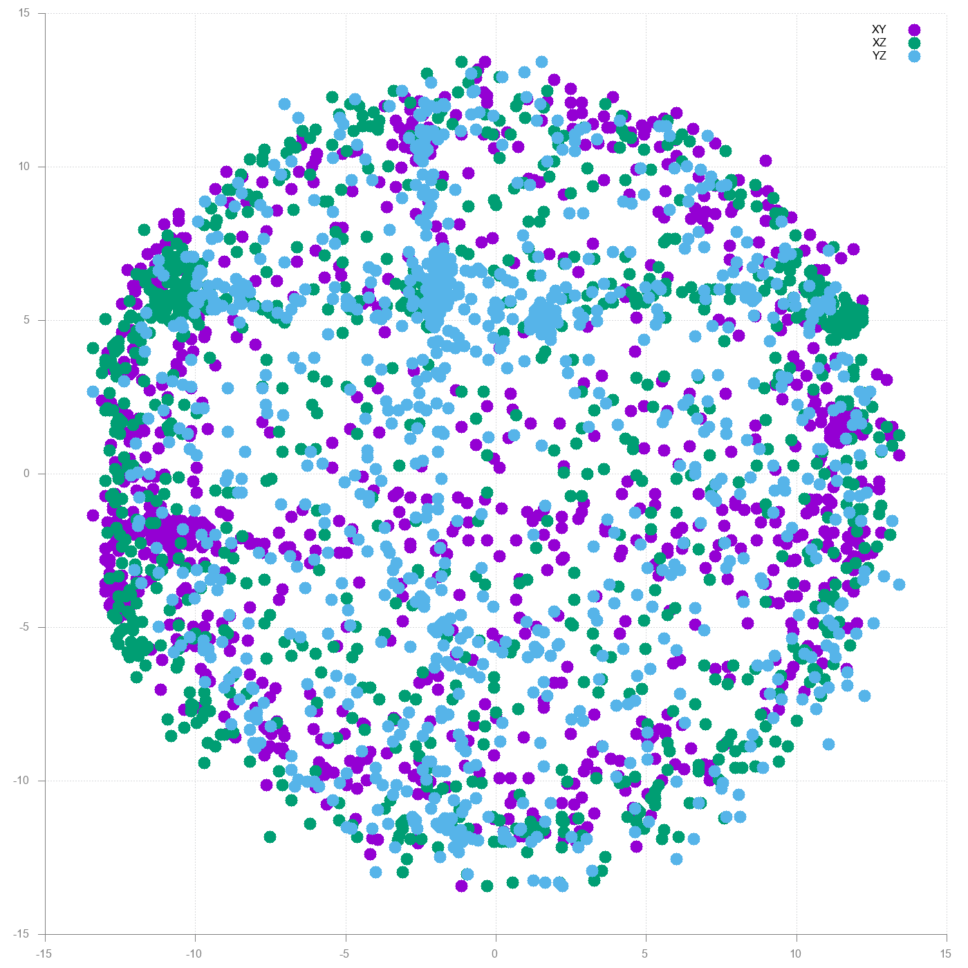
Result already looks how it should look; three spheres centered around 0,0. There is still some distortion so let’s see what the soft iron removal does.
#!/usr/local/bin/python3

import csv
import sys

reader = csv.reader(iter(sys.stdin.readline, ""), delimiter=",")
data = list(reader)

x = [float(row[0]) for row in data]
y = [float(row[1]) for row in data]
z = [float(row[2]) for row in data]

avg_delta_x = (max(x) - min(x)) / 2
avg_delta_y = (max(y) - min(y)) / 2
avg_delta_z = (max(z) - min(z)) / 2

avg_delta = (avg_delta_x + avg_delta_y + avg_delta_z) / 3

scale_x = avg_delta / avg_delta_x
scale_y = avg_delta / avg_delta_y
scale_z = avg_delta / avg_delta_z

for row in data:
    corrected_x = float(row[0]) * scale_x
    corrected_y = float(row[1]) * scale_x
    corrected_z = float(row[2]) * scale_x

    print(",".join(format(value, ".15f") for value in [corrected_x, corrected_y, corrected_z]))
Run this script using the hard iron corrected values as input.
$ ./softiron.py < hardiron.csv > softiron.csv
Plot the graph again.
gnuplot> plot "softiron.csv" using 1:2 title "XY" pointsize 2 pointtype 7, \
              "softiron.csv" using 1:3 title "XZ" pointsize 2 pointtype 7, \
              "softiron.csv" using 2:3 title "YZ" pointsize 2 pointtype 7
On the first sight difference is not that big. However if you look closer the dots create a bit better formed sphere than before.
Additional reading
Simple and Effective Magnetometer Calibration by Kris Winer which is basis for this blog post. Rest of the wiki is good reading too.
A Way to Calibrate a Magnetometer by Teslabs for more indepth dive on mathematics. Also has example code on how to calibrate using ellipsoid fitting.
Magnetometer Offset Cancellation: Theory and Implementation by William Premerlani describes alternative method for Magnetometer calibrating which can be done on the fly. This is also used in several drone flight controllers.
Calibrating an eCompass in the Presence of Hard- and Soft-Iron Interference ie. the Freescale Semiconductor Application Note AN4246.